Genuine Sieve of Eratosthenes with Elm Generators
I recently worked on a generator library for Elm (to simulate laziness and work with streams). Since I ended up publishing it as a package, I needed some examples and dug up the Sieve of Eratosthenes.
Sieve of Eratosthenes
The Ancient Greek algorithm provides a simple way to eliminate composite numbers (or sieve them out), leaving only the primes. Given the natural numbers > 1…
- two is the first prime number; cross out multiples of two [2, 4, 6…]
- the next number that is not crossed out – three – must be a prime; cross out multiples of three [3, 6, 9…]
- etc
Implementation Considerations
How should the algorithm be implemented? In an imperative language with efficient side effects (e.g. array read writes), multiples can be crossed off all at once (though a finite upper bound must be specified).
In purely functional contexts, a typical solution uses laziness with infinite recursion, e.g. from the Haskell Wiki:
import Data.List.Ordered (minus, union, unionAll)

primes = 2 : 3 : minus [5,7..] (unionAll [[p*p, p*p+2*p..] | p <- tail primes]
In Elm 0.19, as far as I can tell, such infinitely recursive formulations are impossible with the strict compiler. Using generators, though, we can still implement a genuine, infinite sieve.
Algorithm
An algorithm for a purely functional, incremental sieve is described in section 3 of Melissa O’Neill’s paper, The Genuine Sieve of Eratosthenes.
The idea is store the next known composite in a map. As larger candidates are explored and the known composites are found, the map is updated to reflect the next known composites (in a “just-in-time” manner). (A step-by-step illustration follows later in this post.)
The Haskell implementation from the article for an initial version is relatively clear:
sieve xs = sieve’ xs Map.empty
    where
      sieve’ [] table = []
      sieve’ (x:xs) table =
          case Map.lookup x table of
              Nothing −> x : sieve’ xs (Map.insert (x*x) [x] table)
              Just facts −> sieve’ xs (foldl reinsert (Map.delete x table) facts)
            where
                reinsert table prime = Map.insertWith (++) (x+prime) [prime] table
The Elm version incorporates a few optimizations noted in the article, including the fact that different “wheels” may be used to generate candidates.
- trivially, start with 2 and only try odd numbers [3, 5, 7…], thereby excluding composites involving 2 (referred to as “wheel2”)
- similarly, start with the first primes 2, 3, 5 and only try numbers that are not their composites [7, 11, 13…] (referred to as “wheel2357”)
O’Neill’s paper provides a cycle that can be used to implement a wheel that excludes multiples of 2, 3, 5, and 7.
The core of the Elm version is the recursive function that advances the prime number generator one step (thereby emitting the next prime and updating the map of composites). The logic is the same as the Haskell version above. Here, wheel is itself a generator, emitting candidates to be verified.
sieveNext : SieveState b -> Maybe ( Int, SieveState b )
sieveNext ( map, wheel ) =
    let
        ( guess, wheel_ ) =
            safeAdvance1 wheel
    in
    case Dict.get guess map of
        Nothing ->
            Just
                ( guess, ( insertNext guess wheel_ map, wheel_ ) )

        Just composites ->
            sieveNext
                ( updateMap guess composites map, wheel_ )
Running elm repl on a modern dual-core laptop, the millionth prime can be found in under a minute.
> import Generator as G

> import Examples.Eratosthenes as E

> E.wheel2357Init |> E.sieve |> G.take 10
[2,3,5,7,11,13,17,19,23,29]
    : List Int

> E.wheel2357Init |> E.sieve |> G.drop 999999 |> G.take 1
[15485863] : List Int
Observing the Algorithm
A benefit of using a generator is the ease of observability of internal state at each step.
Using the wheel of odd numbers only, the first two steps yields the first prime, 2, and the second prime, 3, at which point the composite map has been initialized. For the prime 3, the map is keyed at 3 * 3 (since smaller composites will have been previously checked), with a value being another generator for 3 * the wheel candidates, i.e. only the multiples of 3 that will be checked by the algorithm.
> E.wheel2Init |> E.sieve |> G.advance 2

( [2, 3]
, Active
    { next = <function>
    , state = ( ( Dict.fromList [ (9, [Active { next = <function>, state = ((),3) }])
                                ]
                , Active { next = <function>, state = ((),3) }
                )
              , [3]
              )
     }
)
Advancing a few steps, we see that the algorithm has moved past 9, the first composite in the map. Accordingly, the first key in the map has been updated to 15, to reflect the next multiple of 3 to be verified (3 * 5). Other squares of found primes (5, 7, 11) have also been added to the map, with their respective composite generators.
> E.wheel2Init |> E.sieve |> G.advance 5
( [2,3,5,7,11]
, Active
    { next = <function>
    , state = ( ( Dict.fromList [ (15,[Active { next = <function>, state = ((),5) }])
                                , (25,[Active { next = <function>, state = ((),5) }])
                                , (49,[Active { next = <function>, state = ((),7) }])
                                , (121,[Active { next = <function>, state = ((),11) }])
                                ]
                , Active { next = <function>, state = ((),11) })
              , []
              )
    }
)
But we can do better. Since we’re already in Elm, why not feed the data directly into a visualization? (No need to bother with cumbersome serialization / deserialization to and from some non-native data structure.)
Visualizing the Algorithm
A simple visualization is hosted here.
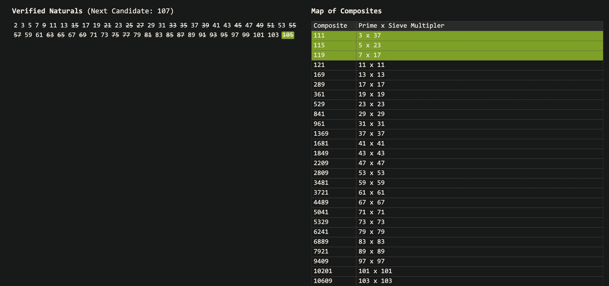
Since the goai is to facilitate the understanding of the sieve and composite map state at each step, the information is presented directly with tables, with highlighting to denote changes from the previous step.
In the below screenshot, we see that with wheel2, 105 has multiple prime factors 3, 5, 7 – all of which have just been updated in the map to their next composites, highlighted in green.